NeuroSorter-Interface: End-to-end spike sorting and cleaning pipeline for neural signals
1. Introduction & Context
The analysis of neural signals is fundamental to understanding brain function and developing new therapies in neuroscience. The spike sorting process, which involves identifying and classifying action potentials (spikes) in extracellular recordings, is a key technical challenge for extracting relevant information from large volumes of data.
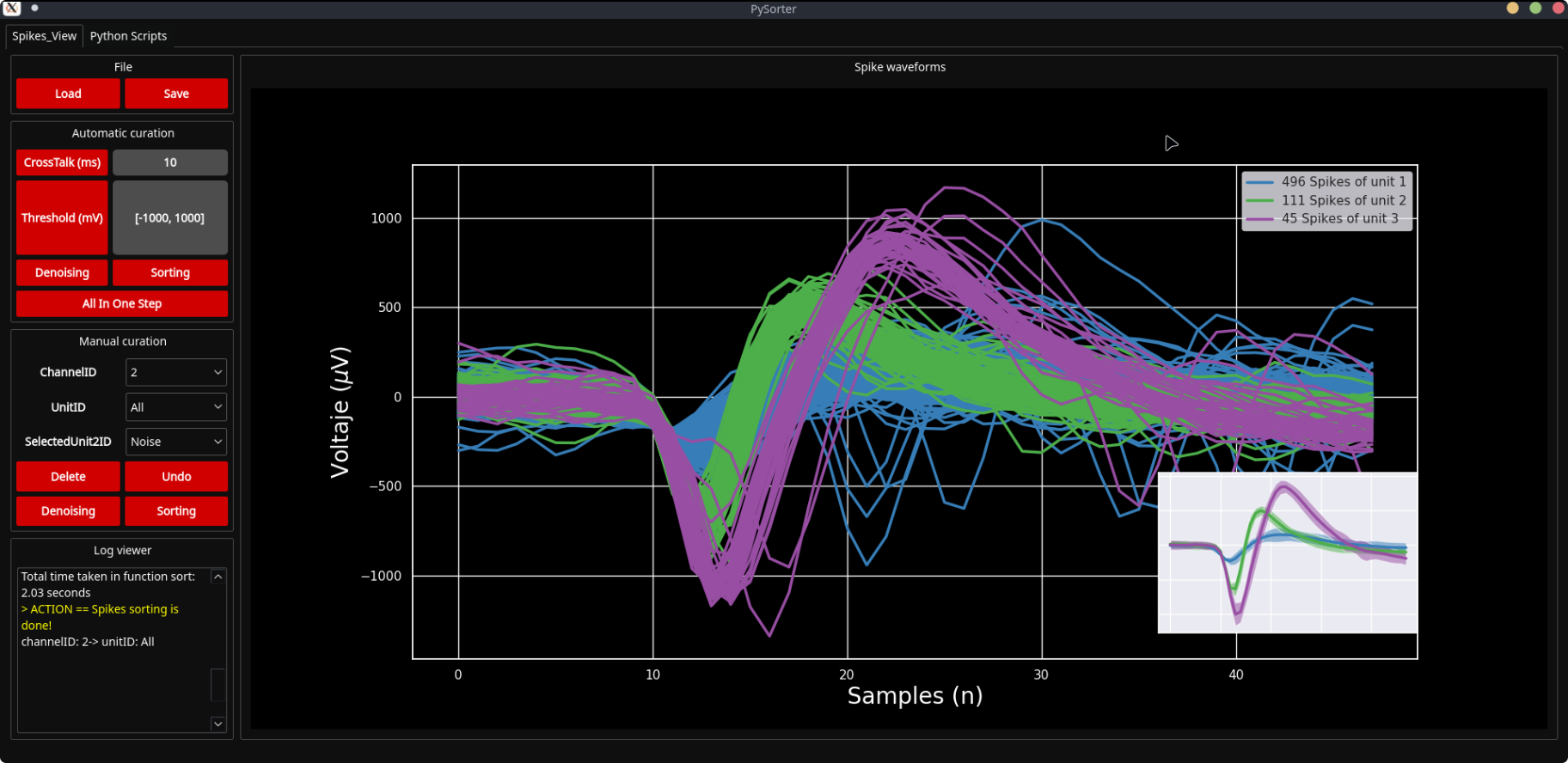
NeuroSorter-Interface emerges as a comprehensive solution for researchers and professionals, enabling efficient cleaning, classification, and visualisation of spikes through advanced algorithms and an intuitive graphical interface. The project connects directly with real neuroscience studies, facilitating the exploration and analysis of experimental data.
2. The Technical Challenge
The main challenge addressed was the automation and robustness of the spike sorting pipeline, dealing with artefacts, noise, and signal variability. Existing solutions tend to be inflexible, require manual intervention, or fail to integrate modern machine learning methods.
NeuroSorter-Interface resolves these limitations by combining dimensionality reduction algorithms (UMAP), clustering (Louvain), and reference templates, all accessible from a GUI that enables dynamic script management and advanced visualisation.
3. The Solution: Architecture
System Modules
- CLEANER: Detection and cleaning of artefacts and spikes using templates and clustering.
- SORTER: Dimensionality reduction (UMAP) and clustering (Louvain) algorithms for automatic classification.
- AUXILIAR_CODE: Auxiliary scripts for specific analyses (ISI, PSTH, raster, etc).
- GUI: PyQt5 graphical interface for interaction, visualisation, and script management.
- DYNAMIC: Dynamic loading and execution of customised scripts.

Pipeline diagram: From raw waveforms to sorted neural units
4. Featured Code
Spike Cleaning and Clustering: A Hybrid Approach
High-Level Architecture
┌────────────────────────────────────────────────────────────────┐
│                         Raw Waveforms                          │
│  Input: N × 48 matrix (N spikes, 48 time samples each)        │
│  Contains genuine spikes + noise + artefacts + outliers       │
└────────────────────┬───────────────────────────────────────────┘
                     │
                     ▼
┌────────────────────────────────────────────────────────────────┐
│                        Normalisation                           │
│  Transform: x_norm = (x - min) / (max - min)                  │
│  Purpose: Scale all waveforms to [0,1] range for consistent   │
│           distance metrics across recordings with different    │
│           amplitudes and baselines                             │
└────────────────────┬───────────────────────────────────────────┘
                     │
                     ▼
┌────────────────────────────────────────────────────────────────┐
│                      UMAP Reduction                            │
│  Transform: ℝ⁴⁸ → ℝ² (48-dimensional → 2-dimensional)         │
│  Algorithm: Uniform Manifold Approximation & Projection        │
│  • Preserves local neighbourhood structure (n_neighbors)      │
│  • Maintains global topology (min_dist)                       │
│  • Manhattan distance metric for spike morphology             │
│  Output: Low-dimensional embedding revealing spike clusters   │
└────────────────────┬───────────────────────────────────────────┘
                     │
                     ▼
┌────────────────────────────────────────────────────────────────┐
│                      Graph Building                            │
│  Construction: k-NN graph from UMAP's fuzzy simplicial set    │
│  • Nodes = individual waveforms                               │
│  • Edges = similarity relationships (weighted)                │
│  • Graph topology encodes manifold structure                  │
│  Purpose: Prepare data structure for community detection      │
└────────────────────┬───────────────────────────────────────────┘
                     │
                     ▼
┌────────────────────────────────────────────────────────────────┐
│                    Louvain Clustering                          │
│  Algorithm: Community detection via modularity optimisation   │
│  • Iteratively merges nodes into communities                  │
│  • Maximises within-cluster connections                       │
│  • Minimises between-cluster connections                      │
│  Output: Initial cluster labels (may contain noise clusters)  │
└────────────────────┬───────────────────────────────────────────┘
                     │
                     ▼
┌────────────────────────────────────────────────────────────────┐
│                    Template Matching                           │
│  Validation: Compare cluster means against reference database │
│  • 115 spike templates (validated neural signals)             │
│  • 12 artefact templates (known noise patterns)               │
│  Metrics: Spearman correlation, DTW distance, trend analysis  │
│  Decision: Accept cluster if passes 5 quality criteria        │
└────────────────────┬───────────────────────────────────────────┘
                     │
                     ▼
┌────────────────────────────────────────────────────────────────┐
│                        Clean Spikes                            │
│  Output: Binary labels (1 = valid spike, 0 = noise/artefact)  │
│  Result: Filtered dataset ready for spike sorting             │
└────────────────────────────────────────────────────────────────┘
Algorithm Summary: The pipeline transforms raw neural recordings through a multi-stage process: first normalising signal amplitudes, then projecting high-dimensional waveforms into a 2D manifold that reveals natural groupings, constructing a similarity graph to capture relationships, detecting communities of similar waveforms, and finally validating clusters against known spike and artefact templates. This hybrid approach combines unsupervised learning (UMAP + Louvain) with supervised validation (template matching) to achieve robust spike cleaning.
Validation Criteria
- Spearman correlation (ρ > 0.7): Shape similarity with templates
- Trend analysis: Linear fit slope within [-2%, 3.5%]
- DTW distance (< 6): Dynamic time warping for phase-space matching
- Cluster stability (std < 0.6): Intra-cluster variability
- Artefact exclusion: High correlation (> 0.95) with noise templates
Spike Sorting Pipeline: Unit Classification and Template Assignment
High-Level Architecture
┌────────────────────────────────────────────────────────────────┐
│                      Clean Spikes (Input)                      │
│  Input: M × 48 matrix (M validated spikes from cleaning)      │
│  Status: Artefacts removed, only genuine neural activity      │
└────────────────────┬───────────────────────────────────────────┘
                     │
                     ▼
┌────────────────────────────────────────────────────────────────┐
│                    Temporal Windowing                          │
│  Extract: Time samples [10:45] from 48-point waveforms        │
│  Purpose: Focus on spike peak region, discard baseline noise  │
│           • Reduces dimensionality (48 → 35 samples)          │
│           • Removes pre/post-spike variability                │
│  Output: M × 35 matrix with spike-relevant features           │
└────────────────────┬───────────────────────────────────────────┘
                     │
                     ▼
┌────────────────────────────────────────────────────────────────┐
│                        Normalisation                           │
│  Transform: x_norm = (x - min) / (max - min)                  │
│  Purpose: Standardise amplitude variations across units       │
│           • Different neurons have different amplitudes       │
│           • Ensures morphology-based (not amplitude) sorting  │
│  Output: Normalised waveforms in [0,1] range                  │
└────────────────────┬───────────────────────────────────────────┘
                     │
                     ▼
┌────────────────────────────────────────────────────────────────┐
│                      UMAP Reduction                            │
│  Transform: ℝ³⁵ → ℝ² (35-dimensional → 2-dimensional)         │
│  Adaptive n_neighbors: min(n_neighbors, ceil(M/n_neighbors))  │
│  • Handles variable dataset sizes automatically               │
│  • Preserves spike morphology relationships                   │
│  • Manhattan metric optimal for temporal waveform features    │
│  Output: 2D embedding where similar units cluster together    │
└────────────────────┬───────────────────────────────────────────┘
                     │
                     ▼
┌────────────────────────────────────────────────────────────────┐
│                      Graph Construction                        │
│  Build: Weighted k-NN graph from UMAP fuzzy simplicial set   │
│  • Edge weights = similarity between spike pairs              │
│  • Graph structure reveals unit boundaries                    │
│  Purpose: Transform geometric embedding into network problem  │
└────────────────────┬───────────────────────────────────────────┘
                     │
                     ▼
┌────────────────────────────────────────────────────────────────┐
│                    Louvain Clustering                          │
│  Algorithm: Modularity-based community detection              │
│  Resolution parameter: 1.1 (balanced granularity)             │
│  • Higher resolution → more clusters (conservative splitting) │
│  • Produces initial unit labels (Unit 1, Unit 2, ...)        │
│  Output: Preliminary unit assignments (pre-refinement)        │
└────────────────────┬───────────────────────────────────────────┘
                     │
                     ▼
┌────────────────────────────────────────────────────────────────┐
│                    Template Matching                           │
│  Database: 115 pre-validated spike templates                  │
│  For each detected unit:                                      │
│    1. Compute unit mean waveform                              │
│    2. Transform to phase space: [waveform, derivative]        │
│    3. Calculate DTW distance to all 115 templates             │
│    4. Assign to closest template (minimum DTW distance)       │
│  Purpose: Map discovered units to canonical spike morphologies│
│  Output: Refined unit IDs based on template library           │
└────────────────────┬───────────────────────────────────────────┘
                     │
                     ▼
┌────────────────────────────────────────────────────────────────┐
│                      Sorted Units (Output)                     │
│  Output: Integer array of unit labels (0-114)                 │
│  Result: Each spike assigned to specific neural unit          │
│  Format: [Unit_23, Unit_45, Unit_23, Unit_12, ...]           │
└────────────────────────────────────────────────────────────────┘
Algorithm Summary: The sorting pipeline operates on pre-cleaned spikes, first extracting the most informative temporal region and normalising amplitudes. UMAP projects waveforms into a low-dimensional space where morphologically similar spikes cluster naturally. Louvain clustering then identifies these groups as putative neural units. Finally, template matching refines unit identities by comparing each cluster's mean waveform against 115 canonical spike shapes using Dynamic Time Warping in phase space. This two-stage approach (unsupervised discovery + supervised assignment) enables both novel unit detection and consistent labelling across recordings.
Key Innovation
- Uses phase-space DTW (waveform + derivative) for template matching
- Robust to temporal shifts and amplitude variability
- Precise discrimination between morphologically similar units
Additional Resources
- Project README — Full documentation and usage examples
- GitHub Repository — Source code and releases
- AUXILIAR_CODE scripts — Advanced analyses (ISI, PSTH, raster)